Maize yield prediction in Eswatini

library(knitr)
opts_chunk$set(tidy.opts = list(width.cutoff = 60))

Introduction

Maize yield information from FAOSTAT is used in this section to design a model for yield prediction based on remotely sensed Z-scored spatial-temporal indices computed previously.

Data

Load necessary packages and data (MODIS indices and reference yields).

rm(list = ls(all=TRUE))
unlink(".RData")
library(dplyr)
library(reshape2)
root <- root <- 'D:/JKUAT/RESEARCH_Projects/Eswatini/Data/'
filename <- paste0(root, "MODIS/outputs/2000_2020_MODIS_st_indices.rds")
#Indices
index <- readRDS(filename)
index <- as.data.frame(index)
filename <- paste0(root, "Yields/FAOSTAT_SZ_maize_yield.csv")
#Yields
ref <- read.csv(filename, stringsAsFactors = F)

temp <- ref[ref$Year >= 2000 & ref$Unit == "tonnes", c("Year","Value")]
colnames(temp)[2] <- "Yield_tonnes"

Merge yield refence data with satellite indices for model training.

df <- merge(index,temp, by="Year")
knitr::kable(df,align = "l")

Year	NDVI	EVI	FPAR	LAI	GPP	Yield_tonnes
2000	0.7411606	0.4212527	NA	NA	0.4953546	112779
2001	0.2562051	-0.0524735	NA	NA	0.1678476	82536
2002	-0.8384683	-0.6522269	NA	NA	-0.0020507	67639
2003	-0.4130928	-0.2029017	-0.0499667	-0.1897696	-1.3033065	69273
2004	0.3985244	-0.1499997	-0.3330661	-0.4115298	-0.5767296	68087
2005	0.5200565	0.3024980	0.0452522	0.1304741	-0.2504898	74540
2006	0.0471496	0.6077305	0.5025639	0.4582647	0.6186566	67127
2007	-1.2828916	-1.0719244	-0.7466142	-0.9988909	-1.3969325	26170
2008	-0.4744662	-0.9791409	-0.9984130	-1.0110070	-0.4620659	60012
2009	0.7286867	0.3894363	0.0913193	0.1342706	0.3988854	75068
2010	0.3278463	0.5995387	-0.0228007	0.0389736	0.2838685	84685
2011	1.3804522	0.3092396	0.2728595	0.8178207	-0.2355459	75418
2012	0.2716715	0.3085555	0.3331407	0.0599877	-0.0508391	81934
2013	0.7041746	0.5348404	0.9638229	0.9420392	0.4789121	118871
2014	0.4316308	0.7035212	0.8211876	0.9991961	1.5665477	119000
2015	-1.0552476	-0.5846196	-0.2758198	-0.2954577	-0.3370502	82000
2016	-3.1728263	-3.5066937	-3.3533974	-3.1888528	-2.5380942	33000
2017	0.0503048	0.3766478	0.8494430	0.8072019	2.2484281	84000
2018	-0.1531849	0.5785767	0.4927239	0.3289629	0.2613869	113000
2019	0.2521144	1.1465457	0.7457823	0.7345936	0.6511760	95000

Modelling

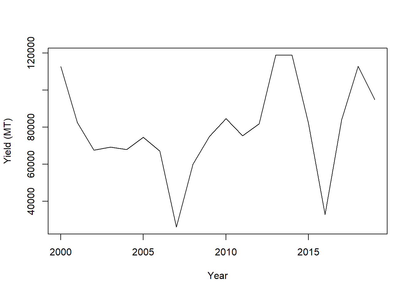
Is there any trends and relationship between predictors and response variables?

Let us make some trend plots from the data:

plot(Yield_tonnes~Year, data=df, xlab="Year", ylab = "Yield (MT)", type='l')

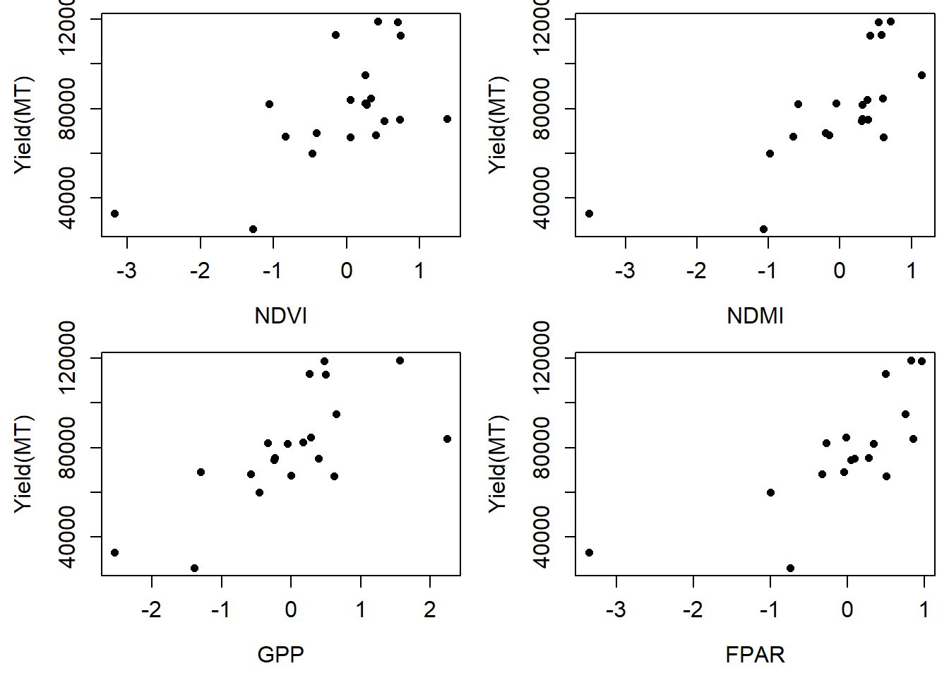
Is there any relationship between for instance NDVI and maize yield in metric tones per hectare?

par(mfrow=c(2,2), mai=c(0.75,0.75,0.1,0.1))
plot(Yield_tonnes~NDVI, data=df, pch=16, ylab= "Yield(MT)", xlab="NDVI", cex=0.9, cex.axis=1.2, cex.lab=1.2)
plot(Yield_tonnes~EVI, data=df, pch=16, ylab= "Yield(MT)", xlab="NDMI", cex=0.9,cex.axis=1.2, cex.lab=1.2)
plot(Yield_tonnes~GPP, data=df, pch=16, ylab= "Yield(MT)", xlab="GPP", cex=0.9, cex.axis=1.2, cex.lab=1.2)
plot(Yield_tonnes~FPAR, data=df, pch=16, ylab= "Yield(MT)", xlab="FPAR", cex=0.9, cex.axis=1.2, cex.lab=1.2)

Relationship between maize yields and satellite metrics.

Feature selection

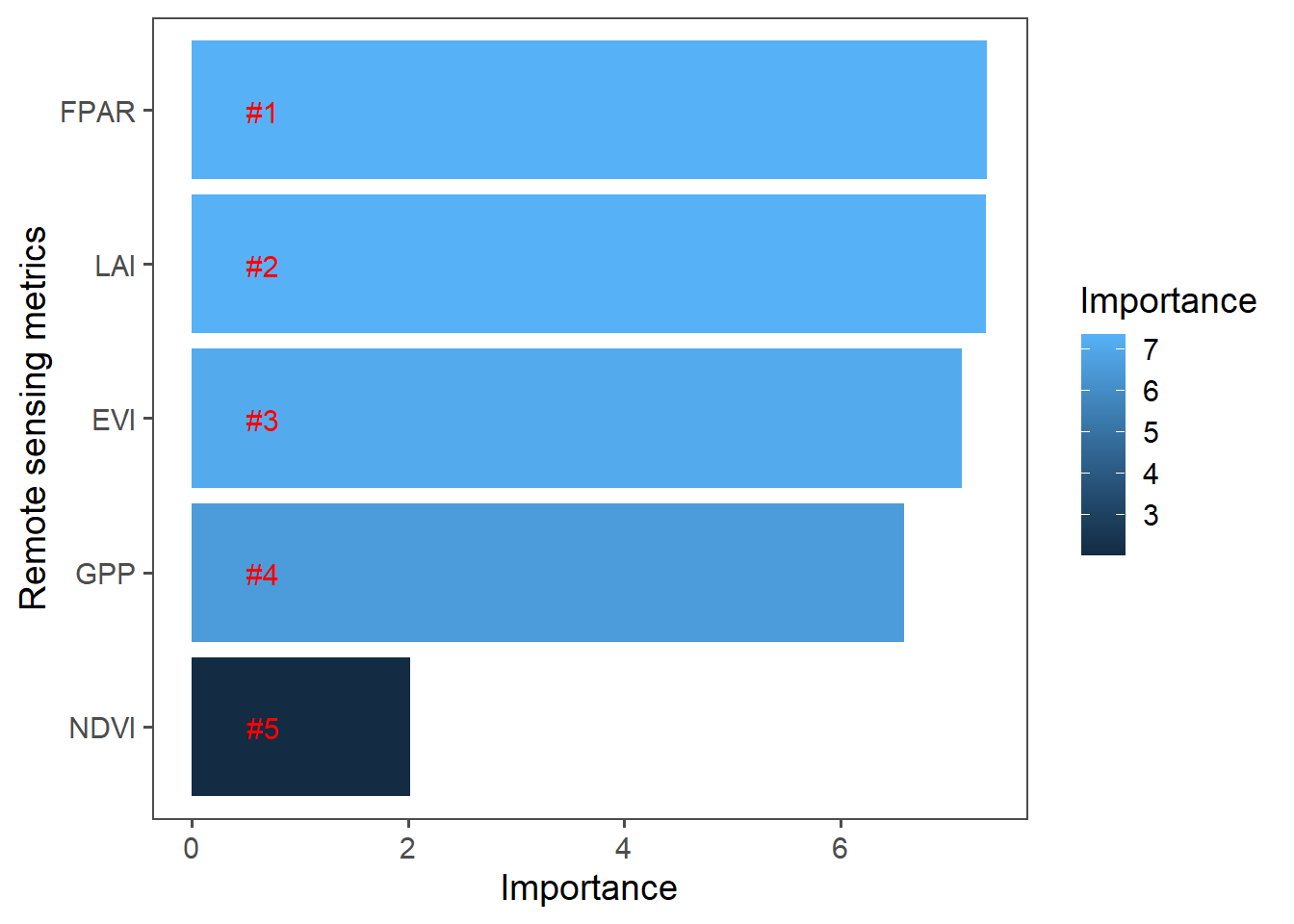
We will use random forest to check the significance of the satellite indices for maize yield prediction.

library(randomForest)

## randomForest 4.6-14

## Type rfNews() to see new features/changes/bug fixes.

## 
## Attaching package: 'randomForest'

## The following object is masked from 'package:dplyr':
## 
##     combine

train <- df

data <- na.omit(df)
rf = randomForest(Yield_tonnes~., data=data[, -1], importance=TRUE, ntree = 500)
importance <- importance(rf)
importance

##       %IncMSE IncNodePurity
## NDVI 2.023014    1598126228
## EVI  7.126598    1709219119
## FPAR 7.355854    1753478416
## LAI  7.348654    1896365793
## GPP  6.589853    1772987638

rf

## 
## Call:
##  randomForest(formula = Yield_tonnes ~ ., data = data[, -1], importance = TRUE,      ntree = 500) 
##                Type of random forest: regression
##                      Number of trees: 500
## No. of variables tried at each split: 1
## 
##           Mean of squared residuals: 363342792
##                     % Var explained: 40.22

varImportance <- data.frame(Variables = row.names(importance), 
                            Importance = round(importance[ ,'%IncMSE'],2))

#Create a rank variable based on importance
rankImportance <- varImportance %>%
  mutate(Rank = paste0('#',dense_rank(desc(Importance))))

#Use ggplot2 to visualize the relative importance of variables
library(ggthemes)
library(ggplot2)

## 
## Attaching package: 'ggplot2'

## The following object is masked from 'package:randomForest':
## 
##     margin

ggplot(rankImportance, aes(x = reorder(Variables, Importance), 
                           y = Importance, fill = Importance)) +
  geom_bar(stat='identity') + 
  geom_text(aes(x = Variables, y = 0.5, label = Rank),
            hjust=0, vjust=0.55, size = 4, colour = 'red') +
  labs(x = 'Remote sensing metrics') +
  coord_flip() + 
  theme_few(base_size = 14)

From Figure @ref(fig:m3) there seems to be some relationship i.e. yields increases with increase in vegetation indices So let us predict 2020 yields using 2003-2019 indices and reference yields.

train <- data[data$Year <= 2013, ] #Training data
newdata <- data[data$Year > 2013, ]
#poly model
train <- train[, -1]

p.lm <- lm(Yield_tonnes~., data=train)
summary(p.lm)

## 
## Call:
## lm(formula = Yield_tonnes ~ ., data = train)
## 
## Residuals:
##        4        5        6        7        8        9       10       11 
##  10989.8  -3511.2    166.7 -14191.8 -12235.2  12032.8  -9583.4  14509.2 
##       12       13       14 
##  -7459.9  -5831.1  15114.0 
## 
## Coefficients:
##             Estimate Std. Error t value Pr(>|t|)    
## (Intercept)    70736       6902  10.249 0.000152 ***
## NDVI           20383      16814   1.212 0.279552    
## EVI           -11609      23716  -0.490 0.645201    
## FPAR           51831      38814   1.335 0.239320    
## LAI           -30351      38508  -0.788 0.466299    
## GPP             7334      12361   0.593 0.578817    
## ---
## Signif. codes:  0 '***' 0.001 '**' 0.01 '*' 0.05 '.' 0.1 ' ' 1
## 
## Residual standard error: 15810 on 5 degrees of freedom
## Multiple R-squared:  0.7379, Adjusted R-squared:  0.4758 
## F-statistic: 2.815 on 5 and 5 DF,  p-value: 0.1403

#Random Forest model
rf = randomForest(Yield_tonnes~., data=train, importance=TRUE, ntree = 500)
importance(rf)

##       %IncMSE IncNodePurity
## NDVI 3.775943     760541215
## EVI  4.924809     664381150
## FPAR 4.038208     953335597
## LAI  3.036205     655371315
## GPP  4.337149     796134782

rf

## 
## Call:
##  randomForest(formula = Yield_tonnes ~ ., data = train, importance = TRUE,      ntree = 500) 
##                Type of random forest: regression
##                      Number of trees: 500
## No. of variables tried at each split: 1
## 
##           Mean of squared residuals: 398422113
##                     % Var explained: 8.06

#SVM https://rstudio-pubs-static.s3.amazonaws.com/280840_d4fb4f186d454d5dbce3ba2cbe4bbcdb.html#tune-svm-regression-model
library(e1071)
svm = svm(Yield_tonnes~., data=train, kernel="radial")
svm

## 
## Call:
## svm(formula = Yield_tonnes ~ ., data = train, kernel = "radial")
## 
## 
## Parameters:
##    SVM-Type:  eps-regression 
##  SVM-Kernel:  radial 
##        cost:  1 
##       gamma:  0.2 
##     epsilon:  0.1 
## 
## 
## Number of Support Vectors:  9

#tune result
tuneResult <- tune(method="svm", Yield_tonnes~.,  data = train, ranges = list(epsilon = seq(0,1,0.1), cost = (seq(0.5,8,.5))), kernel="radial"
)
tuneResult

## 
## Parameter tuning of 'svm':
## 
## - sampling method: 10-fold cross validation 
## 
## - best parameters:
##  epsilon cost
##        0  0.5
## 
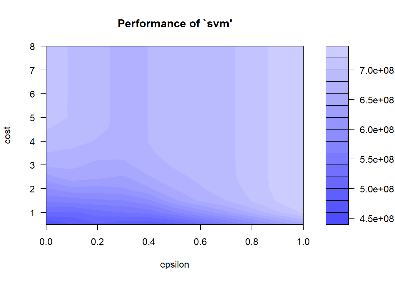
## - best performance: 455161619

plot(tuneResult)

From the SVM tuning graph we can see that the darker the region is the better our model is (because the RMSE is closer to zero in darker regions).

We can use the Root Mean Square Error (RMSE) and mean absolute percentage error (MAPE) to evaluate the models accuracies. RMSE is given as:

\[ \text{RMSE} = \sqrt{\frac{1}{n} \sum_{i=1}^n \widehat{y}-y}, \] where \(\widehat{y}\) and \(y\) are predicted yields and observed yields respectively while n is the number of fitted points.

rmse <- function(error){
  sqrt(mean(error^2))
}

MAPE is given as:

\[ \text{MAPE} = \frac{100\%}{n} \sum_{i=1}^n |\frac{y-\widehat{y}}{y}|. \] In R we can write it as:

MAPE <- function (y_pred, y_true){
    MAPE <- mean(abs((y_true - y_pred)/y_true))
    return(MAPE*100)
}

Let us predict maize yields in the years we left out using the indices based on the model.

lm_y <- predict(p.lm, newdata[,-c(1,7)])
rf_y <- predict(rf, newdata[,-c(1,7)])
svm_y <- predict(svm, newdata[,-c(1,7)])
svm_tuned <- predict(tuneResult$best.model, newdata[,-c(1,7)])

Compute rmse of our predictions.

observed_y <- newdata[, "Yield_tonnes"]
#RMSE from LOESS
rmse(observed_y-lm_y)

## [1] 41067

MAPE(observed_y, lm_y)

## [1] 56.53507

#RMSE from random Forest
rmse(observed_y-rf_y)

## [1] 20048.64

MAPE(observed_y, rf_y)

## [1] 22.38854

#RMSE from SVM not tuned
rmse(observed_y-svm_y)

## [1] 30644.81

MAPE(observed_y, svm_y)

## [1] 40.20859

#RMSE for tuned SVM
rmse(observed_y-svm_tuned)

## [1] 31383.96

MAPE(observed_y,svm_tuned)

## [1] 40.74543

So we choose a model with the lowest RMSE and MAPE and subsequently use it to predict yields in 2020. It also obvious that we would be better off with a high enough data sample. In this case RF model did better and we can use it.

rf <- randomForest(Yield_tonnes~., data=na.omit(df[,-1]), importance=TRUE, ntree = 500)
newdata <- index[index$Year==2020, ]
rf_y <- predict(rf, newdata)
rf_y

##       21 
## 92500.98

The predicted maize yield for the year 2020 is 94010.84 tonnes.

PREVIOUS PAGE.

Created 14th May 2021 Copyright © Benson Kenduiywo, Inc. All rights reserved.