Non-geostatistical prediction
Data
Load the packages and data we will use.
rm(list=ls(all=TRUE))
unlink(".RData")
pacman::p_load(sp, rgdal,rgeos,tmap,raster)
shp <- readOGR("./data/soil_data_CIAT.shp")
plot(shp, pch = 19, col = "red")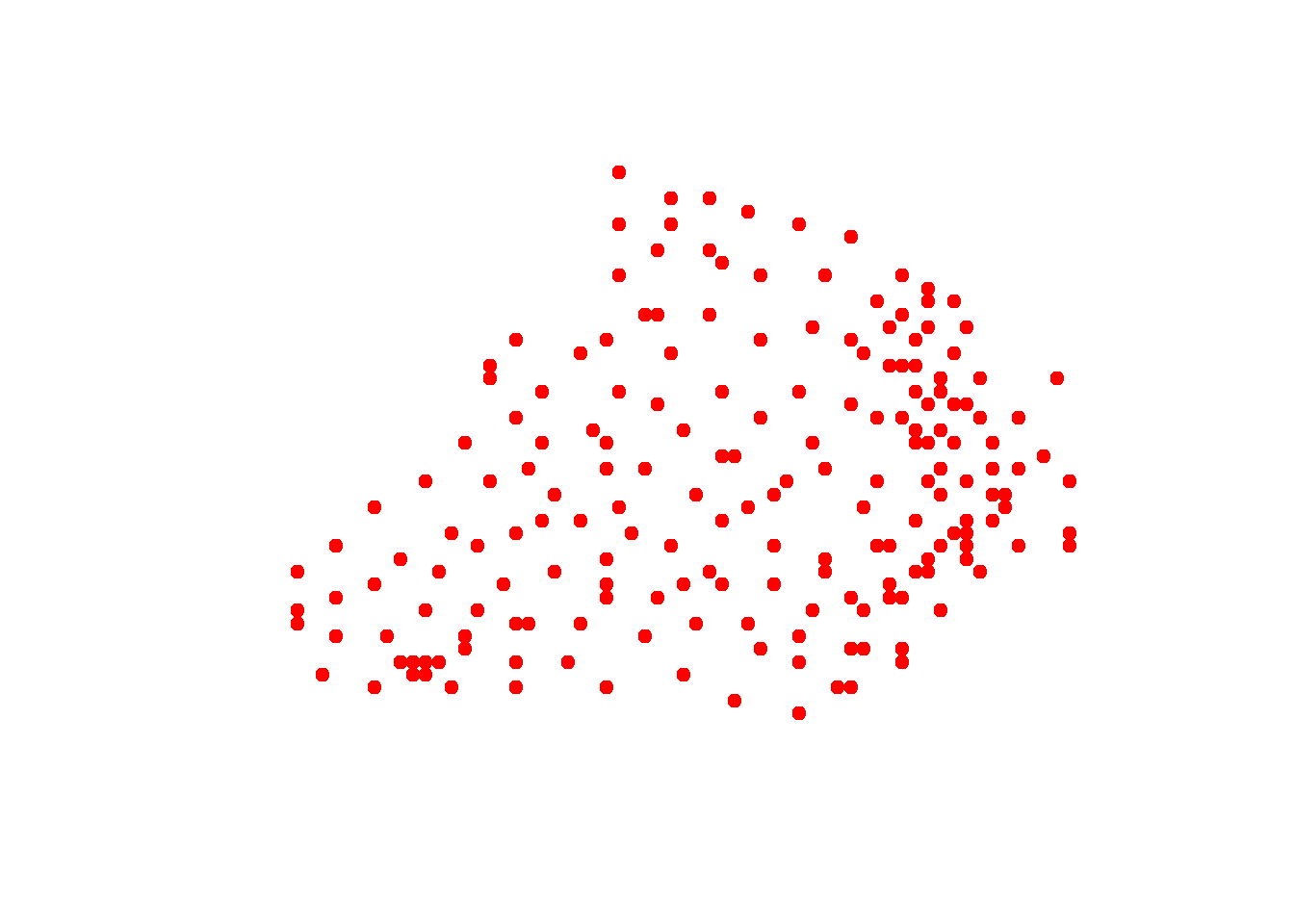
View coordinate reference system and extents of the shapefile.
crs(shp)## CRS arguments:
## +proj=utm +zone=36 +datum=WGS84 +units=m +no_defsextent(shp)## class : Extent
## xmin : 705125
## xmax : 720125
## ymin : 72875
## ymax : 83375Thiessen polygons
- Thiessen polygons are formed to assign boundaries of the areas closest to each unique point. Therefore, for every point in a dataset, it has a corresponding Thiessen polygon.
- We will create Thiessen polygons for the soil data, then use the polygons to map the Clay at their corresponding locations.
- The spatstat package provides the functionality to produce Thiessen polygons via its dirichlet tessellation of spatial point patterns function (dirichlet()).
- We also need to first convert the data to a ppp (point pattern) object class. The maptools package will help us achive this via as.ppp() function.
Load necessary packages and convert data to point pattern.
library(spatstat)  # Used for the dirichlet tessellation function
library(maptools)  # Used for conversion from SPDF to ppp
library(raster)    # Used to clip out thiessen polygons

# Create a tessellated surface
dat.pp <- as(dirichlet(as.ppp(shp)), "SpatialPolygons")
dat.pp <- as(dat.pp,"SpatialPolygons")
Define the projection to the ppp object.
proj4string(dat.pp) <- crs(shp)
plot(dat.pp, pch = 19)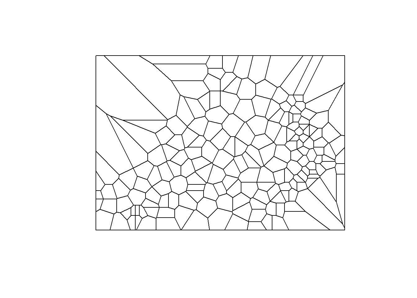
The Polygons are extended beyond points boundary so get the boundary and clip the Thiesen polygon
bdy <- readOGR("./data/soil_boundary.shp")
dat.pp <- intersect(dat.pp, bdy)
plot(dat.pp, pch = 19)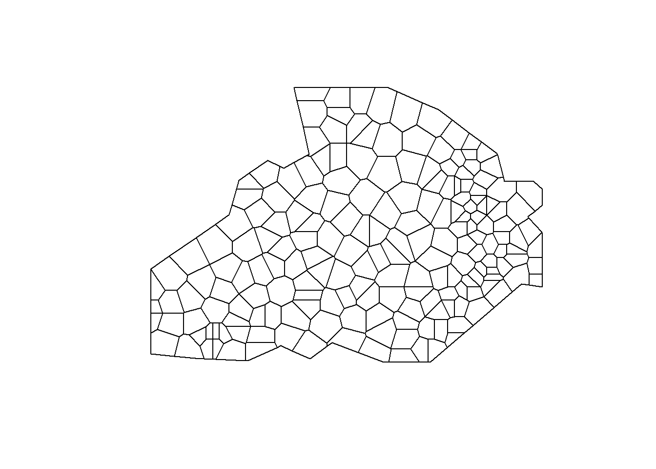
Assign to each polygon the Clay information.
int.Z <- over(dat.pp, shp[,"Clay"], fn=mean, na.rm=TRUE) Map Thiessen polygons and Clay sampled points.
tm_shape(dat.pp) +  tm_borders(alpha=.5, col = "black") +
  tm_shape(shp) + tm_dots(col = "red", scale = 2.5, shape = 16)
## Warning in sp::proj4string(obj): CRS object has comment, which is lost in output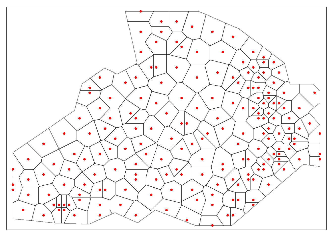
Create a SpatialPolygonsDataFrame object with Clay content,
thiessen <- SpatialPolygonsDataFrame(dat.pp, int.Z)then visualize our point data using the newly formed Thiessen polygons.
tm_shape(thiessen) + tm_fill(col = "Clay", style = "quantile", palette = "Reds", title = "Clay content") + tm_borders(alpha=.3, col = "black") +
tm_shape(shp) + tm_dots(col = "black", scale = 2.5) +
tm_layout(legend.position = c("left", "top"),  legend.text.size = 1.05, legend.title.size = 1.2, frame = FALSE)
## Warning in sp::proj4string(obj): CRS object has comment, which is lost in output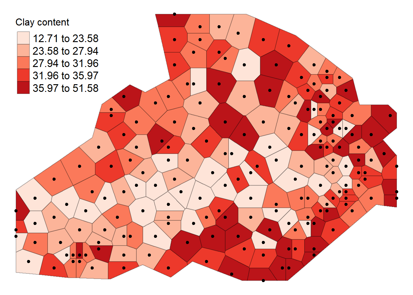
Inverse Distance Weighting (IDW)
- IDW is a means of converting point data of numerical values into a continuous surface to visualise how the data may be distributed across space.
- The technique interpolates point data by using a weighted average of a variable from nearby points to predict the value of that variable for each location (de Smith et al, 2018).
- The weighting of the points is determined by their inverse distances drawing on Tobler’s first law of geography.
Load necessary packages and define sample grid based on the extent of data.
unloadNamespace("spatstat")
pacman::p_load(gstat)
grid <-spsample(bdy, type = 'regular', n = 10000)
## Warning in proj4string(obj): CRS object has comment, which is lost in outputPerform Clay content interpolation using IDW fucntion in Gstat package.
idw <- idw(shp$Clay ~ 1, shp, newdata= grid)## [inverse distance weighted interpolation]Before we visualize the IDW result we transform the data into a data frame object. We can then rename the column headers.
idw.output = as.data.frame(idw)
names(idw.output)[1:3] <- c("long", "lat", "prediction")
Convert the output into a raster in order to visualize the output.
pacman::p_load(raster)
# create spatial points data frame
spg <- idw.output
coordinates(spg) <- ~ long + lat
# coerce to SpatialPixelsDataFrame
gridded(spg) <- TRUE
# coerce to raster
raster_idw <- raster(spg)
# sets projection to British National Grid
projection(raster_idw) <- crs(shp)
we can quickly plot the raster to check if its okay.
plot(raster_idw, main= "Clay content")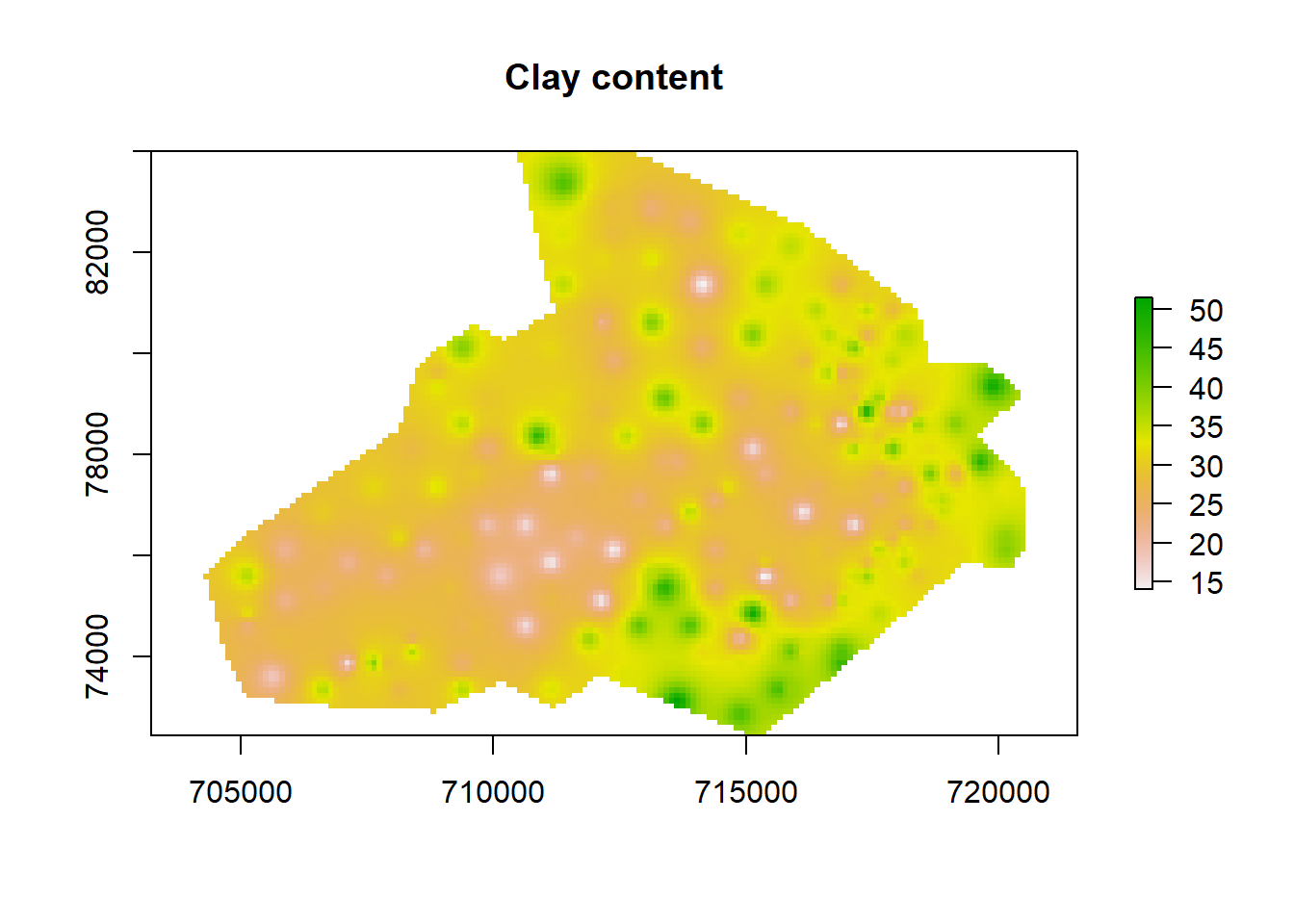
Even 3D plots can be used to visualize the predictions using the raster::persp() function..
persp(raster_idw, col=terrain.colors(100, rev = TRUE))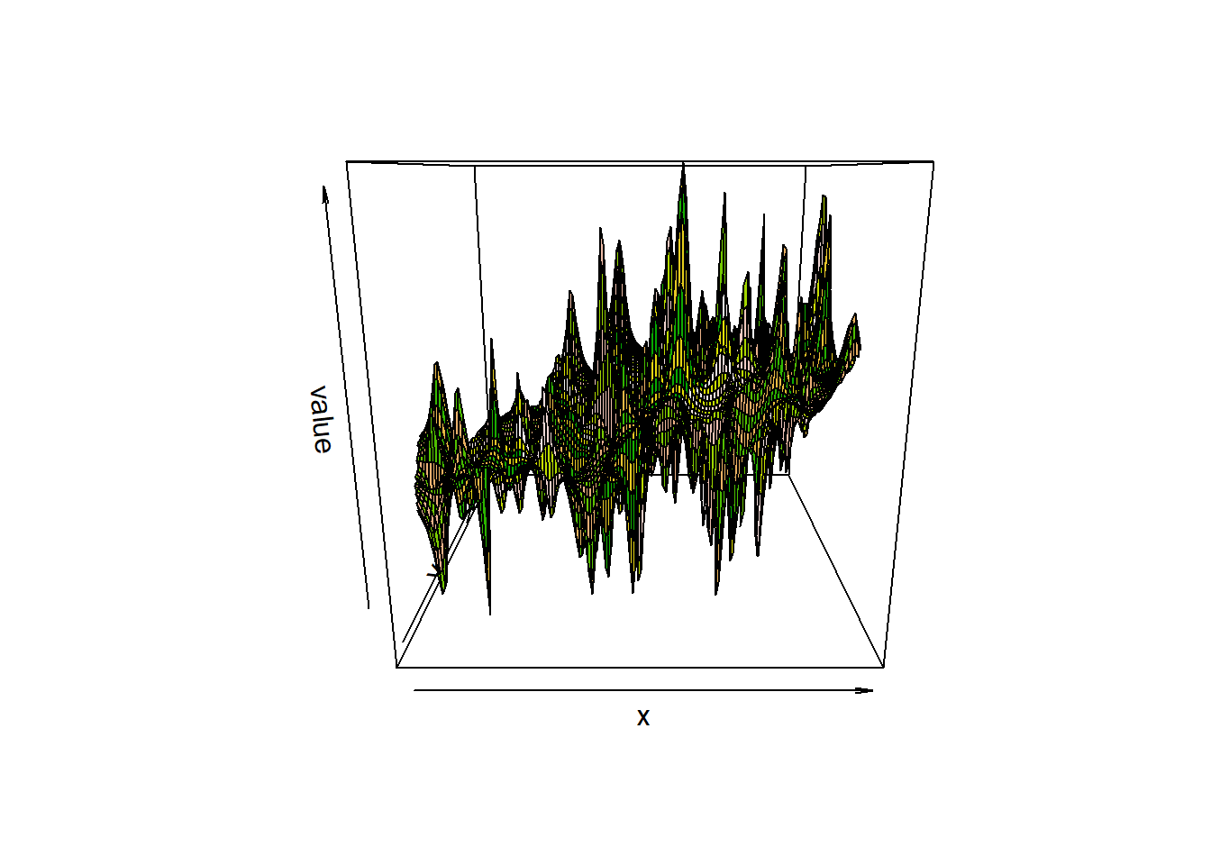
# this package lets us create interactive 3d visualisations
pacman::p_load(rgl)
# we need to first convert the raster to a matrix object type
idw2 <- as.matrix(raster_idw)
persp3d(idw2, col = "red")
Now we are ready to plot the raster. We will use the functionality of the tmap package, using the tm_raster() function. The instructions below will create a smoothed surface. In the example we have created 100 colour breaks and turned the legend off, this will create a smoothed colour effect. You can experiment by changing the breaks (n) to 7 and turning the legend back on (legend.show) to make the predicted values easier to interpret.
pacman::p_load(tmap)
tm_shape(raster_idw) + tm_raster("prediction", style = "quantile", n = 100, palette = "Reds", legend.show = FALSE) +
#Overlay the  boundary to provide some orientation
tm_shape(bdy) + tm_borders(alpha=1, col = "blue")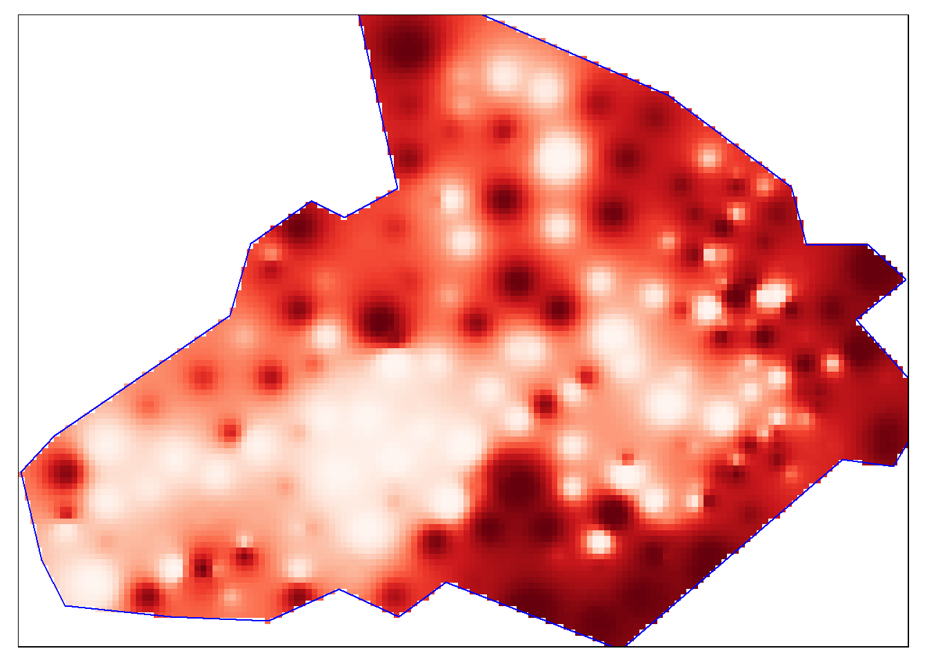
Overlay the original Clay data as this provides a good demonstration of how the IDW is distributed.
tm_shape(raster_idw) + tm_raster("prediction", style = "quantile", n = 100, palette = "-Reds",legend.show = FALSE) +
tm_shape(bdy) + tm_borders(alpha=1, col="black") +
tm_shape(shp) + tm_bubbles(size = "Clay", col = "Clay", palette = "-Purples", contrast=1, style = "quantile", legend.size.show = FALSE, title.col = "Clay content (%)") +
tm_layout(legend.position = c("left", "top"),  legend.text.size = 1.1, legend.title.size = 1.4, frame = FALSE, legend.bg.color = "white", legend.bg.alpha = 0.5)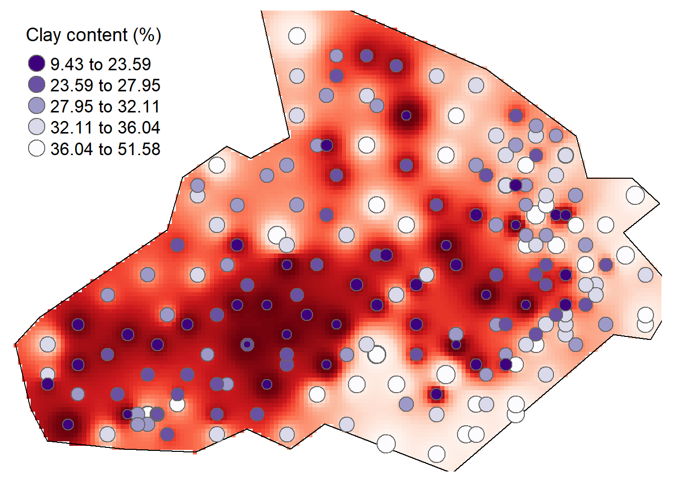
Optimizing IDW predictions
The choice of power function idp can be subjective. To fine-tune the choice of the power parameter, you can perform a leave-one-out cross validation routine to measure the error in the interpolated values.
IDW.out <- vector(length = length(shp))
for (i in 1:length(shp)) {
  IDW.out[i] <- idw(Clay ~ 1, shp[-i,], shp[i,], idp=2.0)$var1.pred
}
Plot the differences in a scatterplot to evaluate accuracy. If not sufficient you can change the idp parameter and evaluate again.
OP <- par(pty="s", mar=c(4,3,0,0))
  plot(IDW.out ~ shp$Clay, asp=1, xlab="Observed", ylab="Predicted", pch=16,
       col=rgb(0,0,0,0.5))
  abline(lm(IDW.out ~ shp$Clay), col="red", lw=2,lty=2)
  abline(0,1)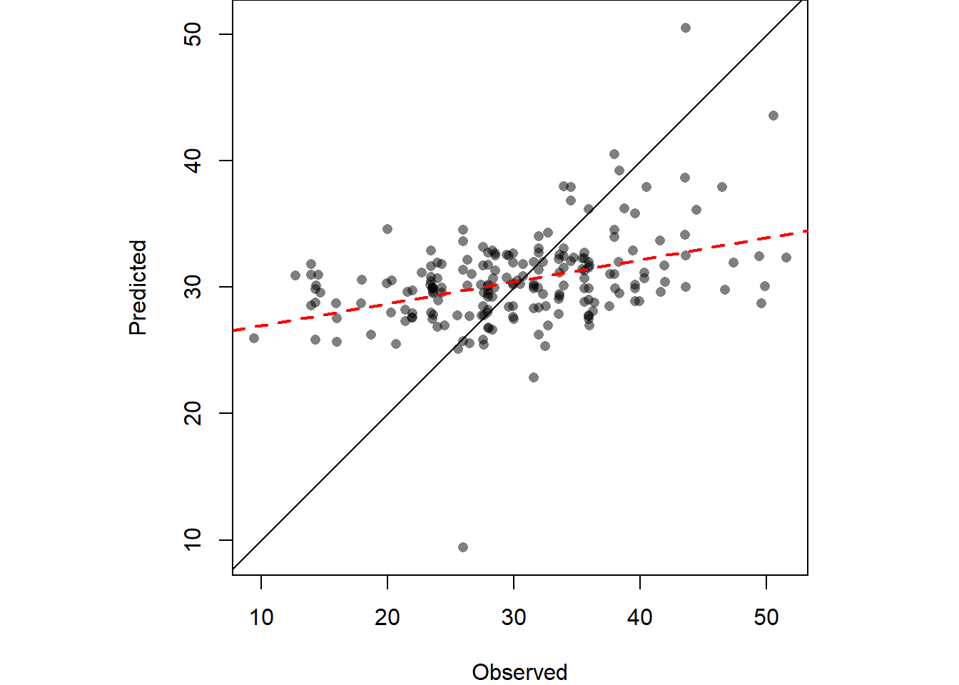
par(OP)We can also compute Root Mean Square Error (RMSE) can be computed from IDW.out.
sqrt( sum((idw.output$prediction - shp$Clay)^2) / length(shp$Clay))## Warning in idw.output$prediction - shp$Clay: longer object length is not a
## multiple of shorter object length## [1] 64.54Cross-validation
We can also create a 95% confidence interval map of the interpolation model to illustrate uncertainity around it. Here we’ll use jackknife technique to estimate a confidence interval at each unsampled point. Frist create an interpolation surface.
img <- gstat::idw(Clay~1, shp, newdata=grid, idp=2.0)## [inverse distance weighted interpolation]n <- length(shp)
Zi <- matrix(nrow = length(img$var1.pred), ncol = n)Leave out a point then perform interpolation (do this n times for each point).
st <- stack()
for (i in 1:n){
  Z1 <- gstat::idw(Clay~1, shp[-i,], newdata=grid, idp=2.0)
  # coerce to SpatialPixelsDataFrame
  gridded(Z1) <- TRUE
  # coerce to raster
  st <- addLayer(st, raster(Z1, layer=1))
  # Calculated pseudo-value Z at j
  Zi[,i] <- n * img$var1.pred - (n-1) * Z1$var1.pred
}
Compute jackknife estimator of parameter Z at location j.
Zj <- as.matrix(apply(Zi, 1, sum, na.rm=T) / n )

# Compute (Zi* - Zj)^2
c1 <- apply(Zi,2,'-',Zj)            # Compute the difference
c1 <- apply(c1^2, 1, sum, na.rm=T ) # Sum the square of the difference

# Compute the confidence interval
CI <- sqrt( 1/(n*(n-1)) * c1)

# Create (CI / interpolated value) raster
gridded(img) <- TRUE
img.sig   <- img
img.sig$v <- CI /img$var1.pred
Clip the confidence raster to boundary and plot the map.
r <- raster(img.sig,  layer="v")
r.m <- mask(r, bdy)

# Plot the map
tm_shape(r.m) + tm_raster(n = 10, style = "kmeans", palette = "-Blues",title="95% confidence interval \n(Clay [%])") +
  tm_shape(shp) + tm_dots(size=0.2) +
  tm_legend(legend.outside=TRUE)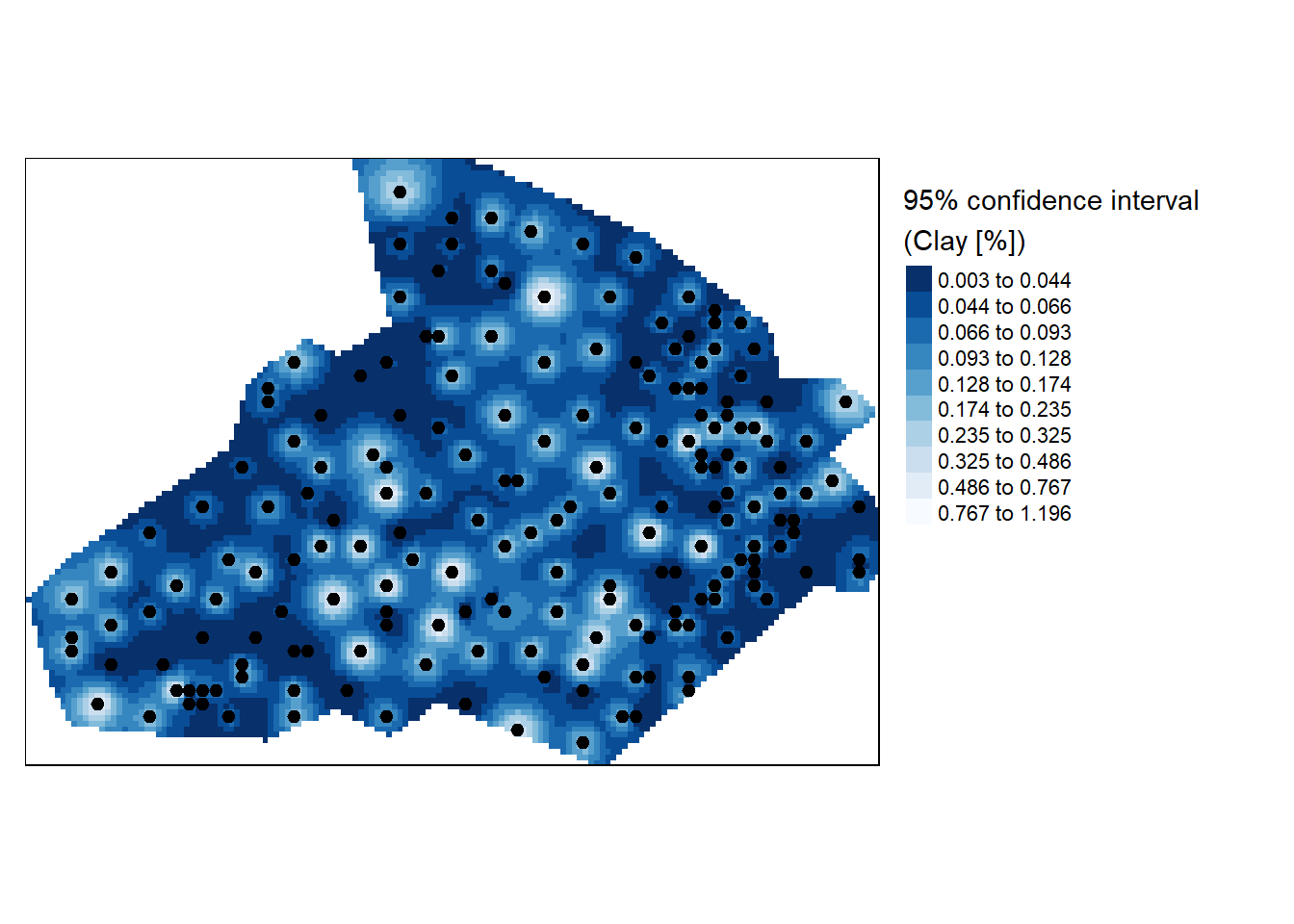
References
De Smith, M. J., Goodchild, M. F., & Longley, P. (2018). Geospatial analysis: a comprehensive guide to principles, techniques and software tools. Troubador publishing ltd.